
Discrete Signals
A very brief overview of discrete vs continuous signals: continuous signals are signals we find in the real world, that are made up of an infinite stream of “samples” or values that are infinitesimally close to each other in time. When we try to measure these real signals, we are constrained by our measuring instruments. A discrete time signal is finite set of samples, which restrains us to knowing the value of the signal at discrete instants in time, and not for all time. For example, take a continuous sine wave:
\[x(t) = sin(2\pi f_0t)\]It’s frequency \(f_0\) is measured in hertz (Hz), which is the number of cycles per second. \(f_0t\) gives the number of cycles in fraction form, and multiplying by \(2\\pi\) gives us the number of cycles in fraction form in radians.
To measure the signal, we must ‘sample’ the continuous time signal and then combine these samples to form the discrete time signal. Below is an example of both the continuous time signal and its sampled version. In the figure, the signal is sampled every \(t_s\) seconds.
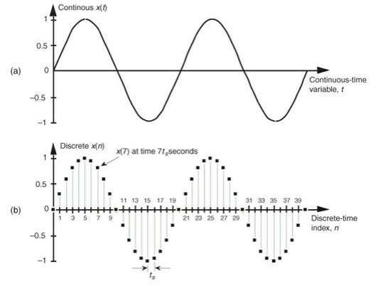 Sine wave - Continuous vs. Discrete
In this post, we will be discussing this sampling operation in more detail, and that is by trying to answer one question: How well does the sampled signal represent the true signal? This is a very important consideration, as if the representation was not good enough, alot of information will be lost, and those losses may be intolerable in some cases.
Signal Ambiguity
Assume we had a 7 Hz sine wave, that we sampled at 6 Hz. That is, six cycles per second for a seven cycles per second signal. We will unavoidably have some information loss since this is a discretization operation in the first place, but here we also risk losing signal representation. Let’s see the result:
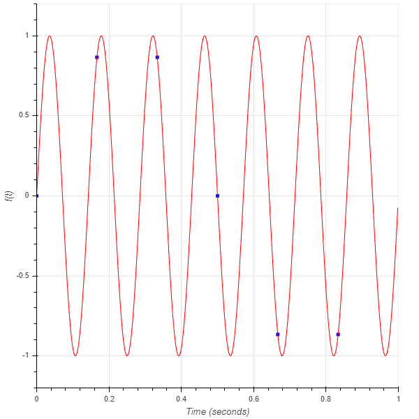 Sampled 7 Hz sine wave at 6 Hz (blue squares), Continuous 7 Hz sine wave (red)
Note that the above continuous signal is not really continuous, just sampled at a much higher rate to make it appear to be for the sake of this example.
So far this seems fine, maybe a not so great representation of our signal, but it doesn’t seem like a deal breaker yet. Now let’s consider another signal sampled at the same rate, specifically a 1 Hz sine wave sampled at 6 Hz. Below is the result:
 Sampled 1 Hz sine wave at 6 Hz (blue squares), Continuous 1 Hz sine wave (red)
This is what the two signal overlayed look like:
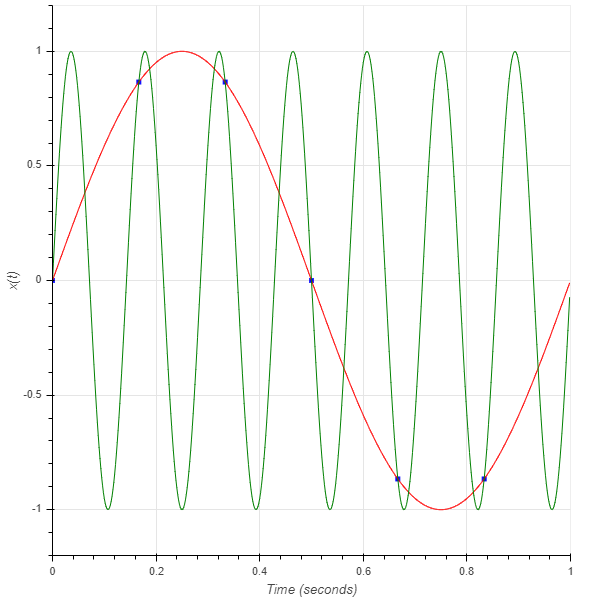 Sampled 1 Hz and 7 Hz sine waves at 6 Hz (blue squares), Continuous 1 Hz and 7 Hz sine waves (red and green accordingly)
Notice that the two signals overlayed have the exact same samples, which we now see is a deal breaker; the two signals, which are of different frequencies, turned out to have the exact same discrete time representation. This is what we call frequency ambiguity, referred to as ALIASING.
In this specific case, we can find a relation for the frequencies that would have the same representation as well, and as it turns out, there are infinitely many. \(x[n]\) is the nth sample of the sampled signal \(x(t)\), which is defined to be \(x[n] = x(nT_s)\) which is simply the nth sample given the sampling period \(T_s\). Also, \(f_s = \frac{1}{T_s}\).
\[x[n] = sin(2\pi f_0nT_s) = sin(2\pi f_0nT_s + 2\pi m) = sin(2\pi nT_s(f_0 + \frac{m}{nT_s})) = sin(2\pi (f_0 + kf_s)nT_s)\]The derived equation tells us that signals with frequencies \(f_0\) Hz and \(f_0 + kf_s\) Hz are indistinguishable given the sampling rate \(f_s\) Hz. This is one of the most important relationships in digital signal processing, upon which all sampling methods are built. Here is another example of misrepresentation of signals and frequency ambiguity:
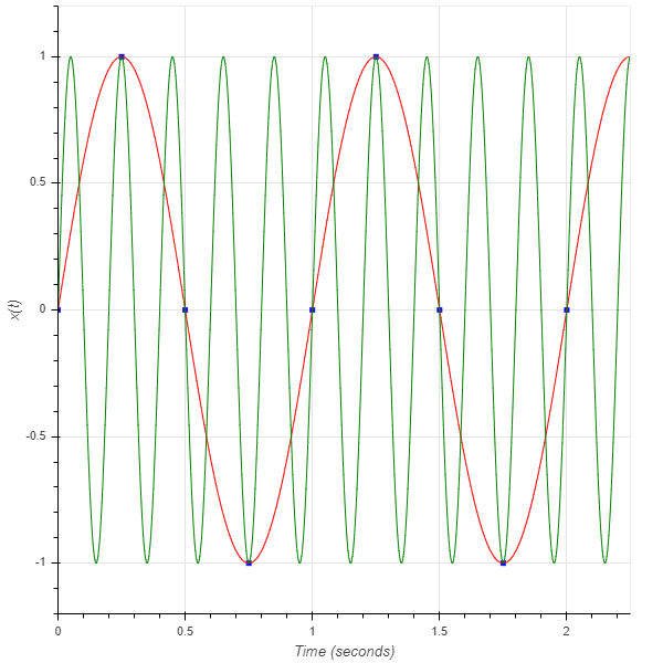 Sampled 1 Hz and 5 Hz sine waves at 4 Hz (blue squares), Continuous 1 Hz and 5 Hz sine waves (red and green accordingly)